Kernel Ridge Regression

library(tidyverse)
set.seed(123)

f <- function(x) sin(3*x) + sin(7*x)
k <- function(x_i, x_j, sigma_f = 0.4, l = 0.4) sigma_f * exp(-(x_i - x_j)^2 / (2 * l^2))

n <- 400
x <- seq(-5, 5, length.out = n)
f_x <- f(x) + rnorm(n, mean = 0, sd = 0.1)

n <- 100
ind_train <- sample(1:400, n, replace = FALSE)
x_train <- x[ind_train]
f_train <- f_x[ind_train]

compute_covmat <- function(k, x, y) {
  n_x <- length(x)
  n_y <- length(y)
  K <- matrix(0, n_x, n_y)
  for (i in 1:n_x) {
    for (j in 1:n_y) {
      K[i, j] <- k(x[i], y[j])
    }
  }
  return(K)
}

k_xx <- compute_covmat(k, x_train, x_train)

lambda <- 0.0001
coef <- solve(k_xx + n * lambda * diag(n)) %*% f_train

f_hat <- function(x) {
  map2_dbl(coef, x_train, ~.x * k(x, .y)) |>
    reduce(`+`)
}

y_hat <- map_dbl(x, f_hat)

colors <- c("Actual" = "blue", "Data" = "black", "Estimate" = "orange")

out <- tibble(x, f = f(x), f_x, y_hat) |>
  pivot_longer(-x) |>
  mutate(
    name = factor(name, levels = c("f", "f_x", "y_hat"), labels = names(colors))
  )
  
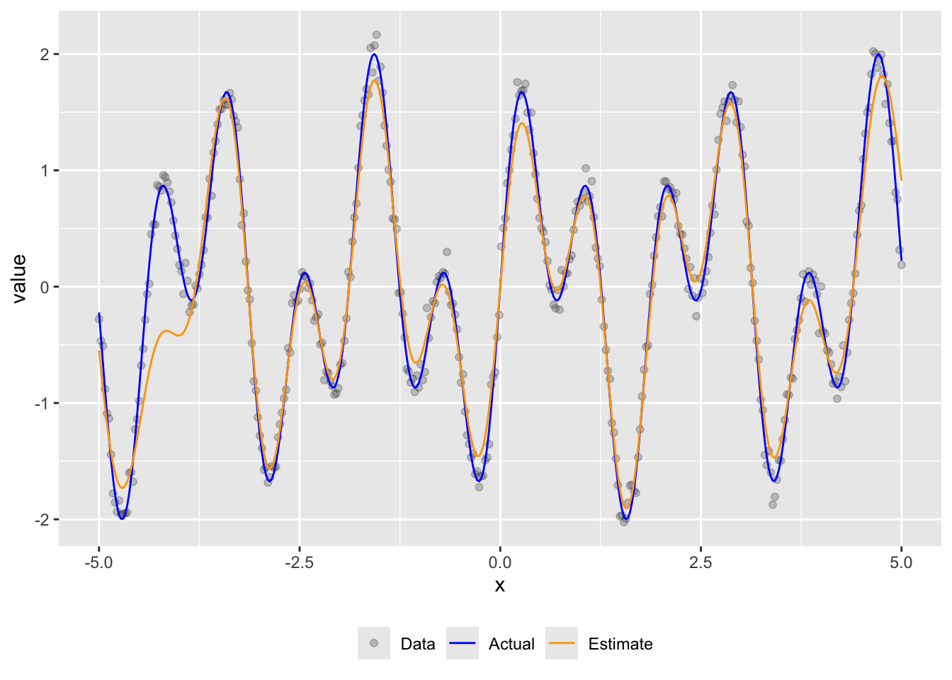
ggplot() +
  geom_point(data = filter(out, name == "Data"), aes(x, y = value, color = name), alpha = 0.2) +
  geom_line(data = filter(out, name == "Actual"), aes(x, y = value, color = name)) +
  geom_line(data = filter(out, name == "Estimate"), aes(x, y = value, color = name)) +
  scale_color_manual(name = "", values = colors) +
  theme(legend.position = "bottom")