Multioutput Gaussian Process Regression (GPR)

Motivation: visualizing vector fields

Elsewhere, I’ve discussed the multivariate normal distribution, and Gaussian processes. Introductory materials discussing Gaussian Processes (GPs) typically focus on univariate outcomes. In more formal notation, input data \(\mathbf{X} \in \mathbb{R}^{N \times P}\) is used to model \(\mathbf{y} \in \mathbb{R}^N\): \[ \begin{align*} \mathbf{y} &= f(\mathbf{X}) + \mathbf{\epsilon} \text{ where } \\ f(\mathbf{X}) &\sim \mathcal{N}_N(\mathbf{0}, \mathbf{K}), \\ \mathbf{\epsilon} &\overset{\text{i.i.d.}}{\sim} \mathcal{N}(0, \sigma_y), \text{ and } \\ \mathbf{K} &= [k(x_i, x_j)]_{ij}^N + \sigma^2_yI_N. \end{align*} \]

Throughout this page, I’ll be using the subscript after \(\mathcal{N}\) to indicate we’re looking at a multivariate normal distribution, and to show the dimension of the vectors that the distribution produces.

While interesting univariate outcomes can be found in abundance, many physical systems and processes are better understood and represented as vectors. In this page, we’ll use the example of the velocity field of hurricane Isabel, which made landfall in 2003. Here is the description of the dataset, from the gcookbook package:

This example and dataset is drawn from The R Graphics Cookbook (Chang 2018), specifically chapter 13.12, on creating vector fields.

This data is from a simulation of hurricane Isabel in 2003. It includes temperature and wind data for a 2139km (east-west) x 2004km (north-south) x 19.8km (vertical) volume. The simluation data is from the National Center for Atmospheric Research, and it was used in the IEEE Visualization 2004 Contest.

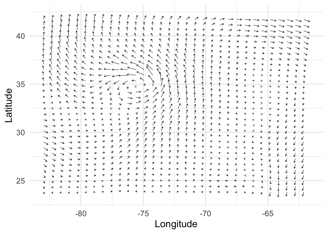
Below I’ve plotted the x and y components of the storm’s velocity field, viewed at approximately 10km above sea-level. Each arrow shows the velocity of the storm’s winds at a given point in the x-y plane. In mathematical notation, we denote the velocity for a particular x-y point as a vector: \[ \mathbf{v} = \begin{bmatrix} v_x \\ v_y \end{bmatrix}. \]

Velocity captures both the direction of the wind, and its magnitude (or strength). Here, longer arrows indicate higher measured speeds. If we wanted, we could plot wind-speed by itself over the area. However, looking only at speed would cause us to miss key dynamics of the phenomena we’re looking at, such as the storm’s spiral shape.

library(tidyverse)
library(gcookbook)
library(scico)
set.seed(123)

eps <- sqrt(.Machine$double.eps)

# Keep a subset in the middle of the the z-axis
d_isabel <- isabel |>
  filter(z == 10.035) |>
  as_tibble()

# Keep 1 out of every 'by' values in vector x
every_n <- function(x, by = 4) {
  x <- sort(x)
  x[seq(1, length(x), by = by)]
}

# Keep 1 of every 4 values in x and y
keep_x <- every_n(unique(isabel$x))
keep_y <- every_n(unique(isabel$y))

# Keep only those rows where x value is in keepx and y value is in keepy
d <- d_isabel |>
  filter(x %in% keep_x, y %in% keep_y) |>
  mutate(index = 1:n())

# Need to load grid for arrow() function
library(grid)

# Set a consistent plotting theme
theme_set(theme_minimal(base_size = 15))

# Make a plot with the subset, and use an arrowhead 0.1 cm long
p0 <- ggplot(d, aes(x, y)) +
  geom_segment(
    aes(xend = x + vx/50, yend = y + vy/50),
    arrow = arrow(length = unit(0.1, "cm")),
    linewidth = 0.25
  ) +
  labs(x = "Longitude", y = "Latitude")

p0

A similar consideration applies to the task of predicting velocity using statistical models. A “naive” approach might be to build a model for each component of velocity. In our case, that would mean finding two functions, \(f_1: \mathbb{R}^2 \to \mathbb{R}\) and \(f_2: \mathbb{R}^2 \to \mathbb{R}\). This amounts to treating \(v_x\) and \(v_y\) as being independent of each other. Depending on context, this may be true according to scientific theory. However, when working with data provided via sensors and instruments, measurement error may move us away from the theoretical ideal.

An improved approach would allow us to incorporate natural information on how our observed target values (each \(v_x\) and \(v_y\)) might interrelate. The approach should also (ideally) account for the fact that we’re trying to predict a vector at a specific point. In other words, we’d like a single function, whose outputs are vector-valued:

\[ \underbrace{\begin{aligned}[c] v_x = f_1\Bigl((x, y)^\top \Bigr) + \epsilon \\ v_y = f_2\Bigl((x, y)^\top \Bigr) + \epsilon \end{aligned}}_{\text{Naive approach}} \qquad\longrightarrow\qquad \underbrace{\begin{aligned}[c] \begin{bmatrix}v_x \\ v_y\end{bmatrix} = f\Bigl((x, y)^\top \Bigr) + \epsilon \end{aligned}}_{\text{Vector-valued approach}} \]

These characteristics are possible within the framework of Gaussian Process Regression, with the goal of modeling multiple outputs simultaneously being referred to as “multioutput”, “multitask”, “cokriging”, or “vector-valued” GP regression. Alvarez, Rosasco, & Lawrence (2012) provides a technical introduction to some of these topics (Alvarez et al. 2012). In the following section, we’ll cover the theory behind the approach as it applies to our example data.

Theory and notation

We are working in the space of the two-dimensional real numbers, \(\mathbb{R}^2\). Let \(S = (\mathbf{X}, \mathbf{Y}) = (x_1, y_1), \dots, (x_N, y_N)\) be our set of training data, where \(x_i, y_i \in \mathbb{R}^2\). It may be convenient to note \(\mathbf{X}, \mathbf{Y} \in \mathbb{R}^{N \times 2}\), and we may refer to \(\mathbf{y} = \text{vec}\ Y \in \mathbb{R}^{2N}\) and \(\mathbf{x} = \text{vec}\ X \in \mathbb{R}^{2N}\). We will use \(\mathbf{X}_* \in \mathbb{R}^{M \times 2}\) to denote a set of test points, for which we want to generate predictions.

We are engaged in a regression task, i.e., we’re attempting to learn the functional relationship \(f\) between \(\mathbf{X}\) and \(\mathbf{Y}\), with an assumption that this relationship has been corrupted to some degree by noise. For the following, I’ve adapted notation from Chapter 2.2 in the well-known Williams and Rasmussen text to the context of our multidimensional \(\mathbf{Y}\) (Williams and Rasmussen 2006). Setting up the problem, we have \[ \begin{align*} \mathbf{y} &= f(\mathbf{x}) + \epsilon \\ f &\sim \mathcal{GP}(m, k) \\ f(\mathbf{x}) &\sim \mathcal{N}_{2N}(\mathbf{0}, \mathbf{K}_{XX}) \end{align*} \tag{1}\]

To parse these statements, we assume \(f\) is drawn from a Gaussian Process with mean function \(m\) and covariance (kernel) function \(k\). Thus, our observations \(\mathbf{y} = f(\mathbf{x})\) have a multivariate normal probability distribution, parameterized by a covariance matrix \(\mathbf{K}_{XX}\). By convention, we assume the mean vector is \(\mathbf{0}\) (implying that \(m\) is the zero function).

The joint distribution of \(\mathbf{y}\) and our predictions for the test point(s) \(\mathbf{y}_*\) is also described by a multivariate normal distribution, specified as: \[ \begin{align*} \begin{bmatrix} \mathbf{y} \\ \mathbf{y_*} \end{bmatrix} &\sim \mathcal{N}_{2N + 2M}\Biggl( \mathbf{0}, \begin{bmatrix} \mathbf{K}_{XX} + \mathbf{V} \otimes \mathbf{I}_N & \mathbf{K}_{XX_*} \\ \mathbf{K}_{X_*X} & \mathbf{K}_{X_* X_*} \end{bmatrix} \Biggr) \\ \mathbf{V} &= \begin{bmatrix} \sigma^2_1 & 0 \\ 0 & \sigma^2_2 \end{bmatrix} \end{align*} \tag{2}\]

Here, \(\sigma^2_1, \sigma^2_2 > 0\) represent the independent and additive noise associated with each of our outcome’s components. The \(\otimes\) symbol denotes the Kronecker product. Each of the sub-matrices, such as \(\mathbf{K}_{XX_*}\), are defined below in Equation 8. From this joint distribution, we can derive the conditional distribution for \(\mathbf{y}_*\):

\[ \begin{align*} \mathbf{y}_* | \mathbf{X}, \mathbf{y}, \mathbf{X_*} &\sim \mathcal{N}_{2M}(\hat{\mu},\ \hat{\mathbf{\Sigma}}) \\ \hat{\mathbf{\mu}} &= \mathbb{E}[\mathbf{y}_* | \mathbf{X}, \mathbf{y}, \mathbf{X_*}] = \mathbf{K}_{X_*X}(\mathbf{K}_{XX} + \mathbf{V} \otimes \mathbf{I}_N)^{-1} \mathbf{y} \\ \hat{\mathbf{\Sigma}} &= \mathbf{K}_{X_*X_*} - \mathbf{K}_{X_*X}(\mathbf{K}_{XX} + \mathbf{V} \otimes \mathbf{I}_N)^{-1}\mathbf{K}_{XX_*} \\ \end{align*} \tag{3}\]

We will now work through how each piece of our distribution is defined. Let \(k: \mathbb{R}^2 \times \mathbb{R}^2 \to \mathbb{R}\) be a (scalar) kernel function, defined as \[ k(x_i, x_j) = \alpha^2 \cdot \exp\Bigl(-\frac{1}{2\rho^2} \| x_i - x_j \|^2 \Bigl), \tag{4}\]

where \(\alpha, \rho > 0\), and \(\| \cdot \|\) is the Euclidean (L2) norm. This is also known as the squared exponential function, or the radial basis function. The parameter \(\alpha\) controls …, while \(\rho\) controls the length-scale. Let \(k(\mathbf{X}, \mathbf{X}) \in \mathbb{R}^{N \times N}\), the covariance matrix between all points in \(\mathbf{X}\), be defined as \[ k(\mathbf{X}, \mathbf{X}) = (k(x_i, x_j))_{i,j}^N = \begin{bmatrix} k(x_1, x_1) & \cdots & k(x_1, x_N) \\ \vdots & \ddots & \vdots \\ k(x_N, x_1) & \cdots & k(x_N, x_N) \end{bmatrix}. \tag{5}\]

Let \(\mathbf{B} \in \mathbb{R}^{2 \times 2}\), the matrix of similarities between the outputs \(\mathbf{Y}\), be defined as \[ \mathbf{B} = \text{corr}(\mathbf{Y}) = \Biggl( \frac{\langle \mathbf{y}_i - \bar{\mathbf{y}}_i,\ \mathbf{y}_j - \bar{\mathbf{y}}_j \rangle}{\| \mathbf{y}_i - \bar{\mathbf{y}}_i \| \| \mathbf{y}_j - \bar{\mathbf{y}}_j \| } \Biggr)^{2,2}_{i,j}, \tag{6}\]

where \(\mathbf{y}_i\) is the i-th column of \(\mathbf{Y}\) and \(\bar{\mathbf{y}}_i\) is the arithmetic mean of \(\mathbf{y}_i\). The operation in the numerator, \(\langle \cdot, \cdot \rangle\), denotes the standard inner product. Each entry \(b_{i,j}\) of \(\mathbf{B}\) is the Pearson correlation coefficient, as estimated from our training data.

Let \(\mathbf{K}_{XX} \in \mathbb{R}^{2N \times 2N}\) be defined as \[ \mathbf{K}_{XX} = \mathbf{B} \otimes k(\mathbf{X}, \mathbf{X}). \tag{7}\]

Alvarez et al. identifies this approach of combining the kernel matrix with a similarity matrix via a Kronecker product as the “Intrinsic Coregionalization Model”; see equation (21) in section 4.2.2 (Alvarez et al. 2012). They describe this approach as being more restrictive, but simpler (to implement, I assume).

We can now define the other pieces needed to establish the covariance matrix used for the joint distribution of \(\begin{bmatrix} \mathbf{y} \\ \mathbf{y}_* \end{bmatrix}\):

\[ \begin{align*} \mathbf{K}_{X_*X_*} &= \mathbf{B} \otimes k(\mathbf{X}_*, \mathbf{X}_*) = \mathbf{B} \otimes (k(x_{*i}, x_{*j}))_{i,j=1}^{M} \in \mathbb{R}^{2M \times 2M} \\ \mathbf{K}_{X_*X} &= \mathbf{B} \otimes k(\mathbf{X}_*, \mathbf{X}) = \mathbf{B} \otimes (k(x_{*i}, x_j))_{i,j=1}^{M,N} \in \mathbb{R}^{2M \times 2N} \\ \mathbf{K}_{XX_*} &= \mathbf{K}_{X_*X}^\top \in \mathbb{R}^{2N \times 2M}. \end{align*} \tag{8}\]

Training and test data

Here, using the Hurricane Isabel data visualized above, we generate \(S\), defined as a 30% random sample of observations. Here d is our subset of the isabel dataset, at z = 10.035.

# Set up the training data
S <- d |>
  slice_sample(n = floor(0.3 * nrow(d))) |>
  select(x, y, vx, vy, index)

X <- S |> select(x, y) |> as.matrix()
Y <- S |> select(vx, vy) |> as.matrix()
y <- as.vector(Y)
B <- cor(Y)
N <- nrow(X)

# Pull out test cases
Z <- d |>
  anti_join(S, by = "index") |>
  select(x, y, vx, vy, index)

X_star <- Z |> select(x, y) |> as.matrix()

Kernel functions

This section defines R functions used to compute \(\mathbf{K}_{XX}\).

#' Squared exponential (scalar) kernel function
#' 
#' @param xi numeric vector
#' @param xj numeric vector
#' @param alpha scale, alpha > 0
#' @param rho length-scale, rho > 0
#' @return numeric
k <- function(xi, xj, alpha = 1, rho = 1) {
  alpha^2 * exp(-norm(xi - xj, type = "2")^2 / (2 * rho^2))
}

#' Compute the kernel matrix, given a set of input vectors
#' 
#' @param X numeric matrix of dimensions N x P, where N is observations and P is components
#' @param alpha numeric, variance scale, alpha > 0
#' @param rho numeric, length-scale, rho > 0
#' @param err numeric, err > 0
#' @return N x N matrix
k_XX <- function(X, alpha = 1, rho = 1, err = eps) {
  N <- nrow(X)
  K <- matrix(0, N, N)
  for (i in 1:N) {
    for (j in 1:N) {
      K[i, j] <- k(X[i, ], X[j, ], alpha, rho)
    }
  }

  if (!is.null(err)) {
    K <- K + diag(err, ncol(K))
  }

  K
}

#' Compute the covariance between two sets of vectors
#'
#' @param x numeric matrix, N x P
#' @param X numeric matrix, M x P
#' @param alpha numeric, variance scale, alpha > 0
#' @param rho numeric, length-scale, rho > 0
#' @return A numeric matrix, N x M
k_xX <- function(x, X, alpha = 1, rho = 1) {
  N <- nrow(x)
  M <- nrow(X)

  K <- matrix(0, N, M)
  for (i in 1:N) {
    for (j in 1:M) {
      K[i, j] <- k(x[i, ], X[j, ], alpha, rho)
    }
  }

  K
}

Hyperparameter Inference

Estimation via Stan

This section contains the rstan code used to estimate hyperparameter values using the probabilistic programming language, Stan. Within the scoped blocks of the Stan program we establish the model for \(f(x)\) discussed in Equation 1, and attempt to find plausible values for \(\rho\) and \(\alpha\) via Hamiltonian Monte-Carlo (HMC). We place prior distributions on each hyperparameter. Constraints are used within Stan to require these parameters be > 0.

library(rstan)

fit_stan <- function(filepath, model_name = "", data, verbose = FALSE) {
  stan(
    file = filepath,
    model_name = model_name,
    data = data,
    chains = 2,
    iter = 800,
    warmup = 400,
    seed = 123,
    cores = 2,
    verbose = verbose
  )
}

# ICM
# fit_stan("./icm.stan", "Isabel GPR, ICM: rho", lst(N, X, Y, B))
# fit_stan("./icm_w_alpha.stan", "Isabel GPR, ICM: alpha & rho", lst(N, X, Y, B))
# fit_stan("./icm_w_alpha_and_sigma.stan", "Isabel GPR, ICM: alpha, rho, & sigma", lst(N, X, Y, B))

# Independent GPs
# fit_stan("./icm.stan", "Isabel GPR, Indep: rho", lst(N, X, Y, B = diag(1, 2)))
# fit_stan("./icm_w_alpha.stan", "Isabel GPR, Indep: alpha & rho", lst(N, X, Y, B = diag(1, 2)))
fit_stan("./icm_w_alpha_and_sigma.stan", "Isabel GPR, Indep: alpha, rho, & sigma", lst(N, X, Y, B = diag(1, 2)))

Evaluation

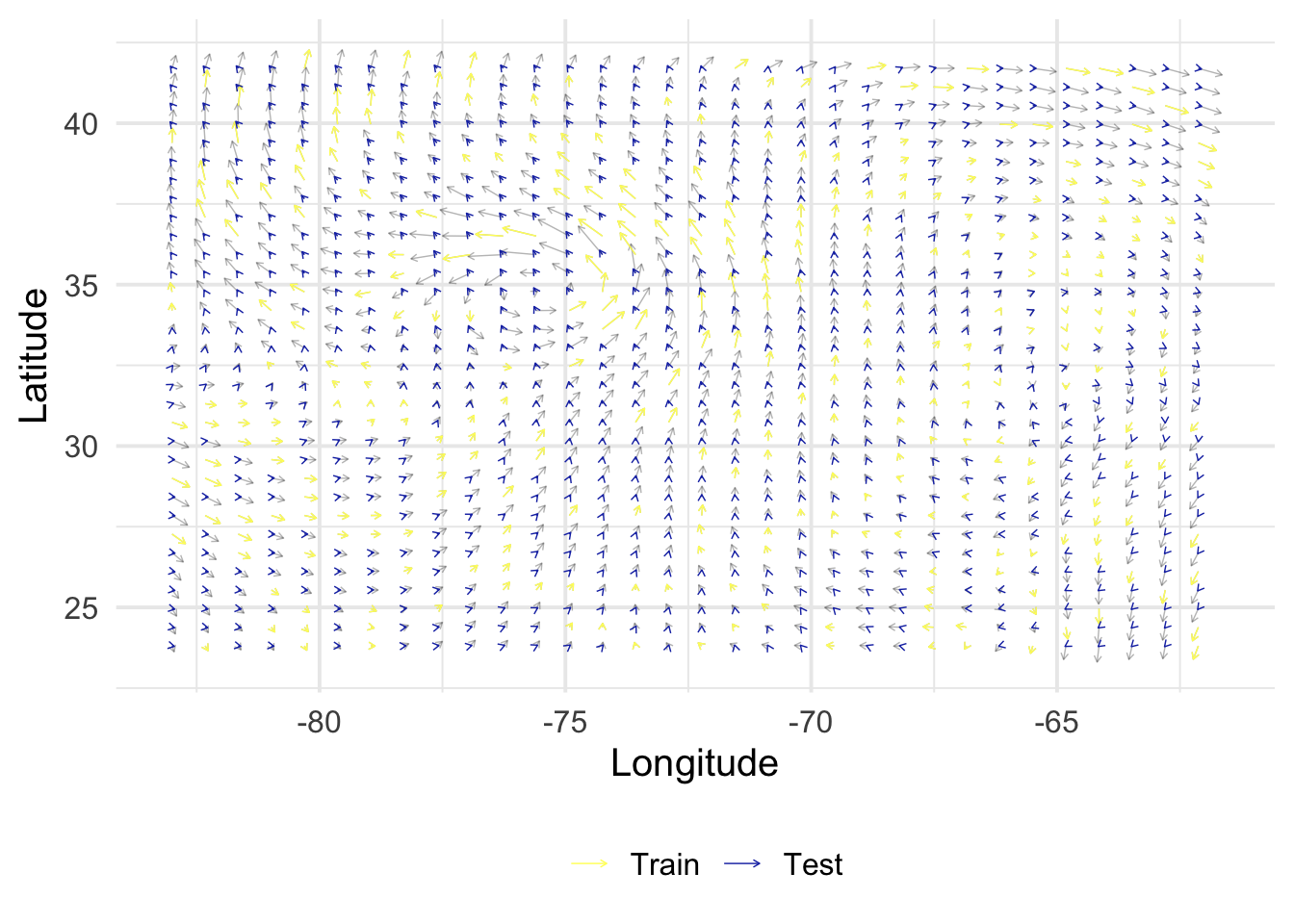
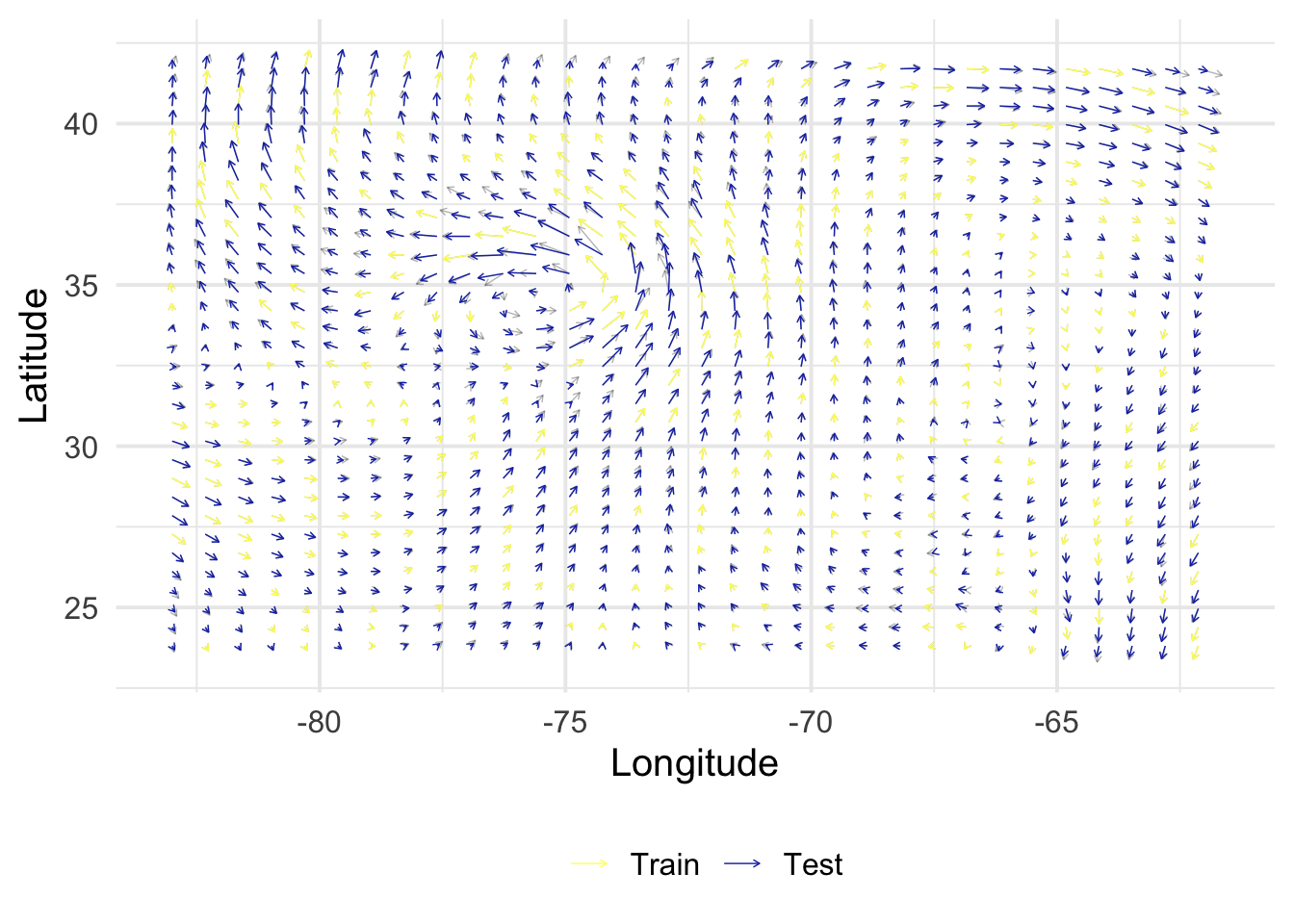
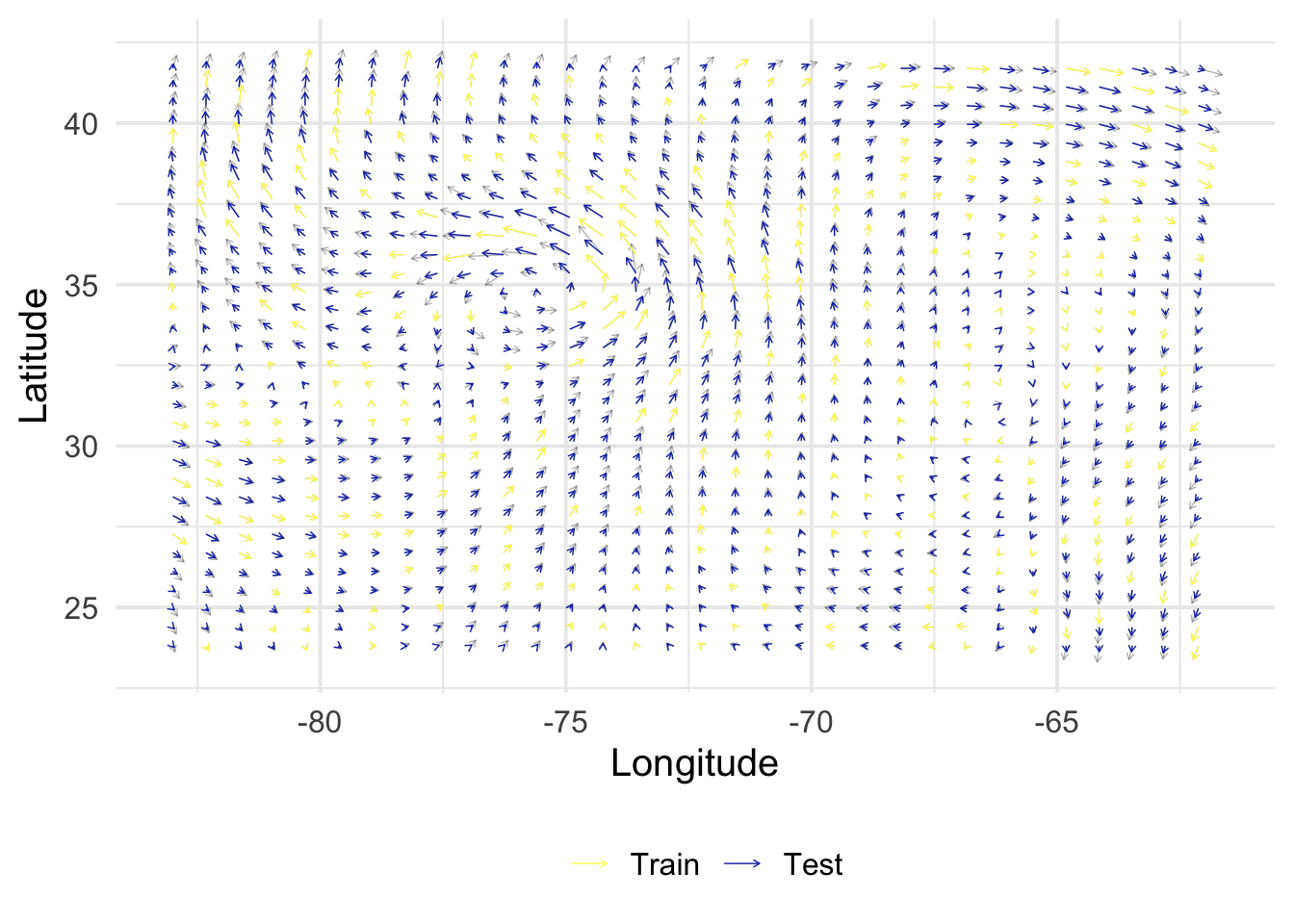
This section defines R functions used to compute the analytical posterior distribution for each parameter specification, and summarize the results with a figure and performance with respect to RMSE.

get_posterior <- function(X, y, B, Z, alpha = 1, rho = 1, sigma = c(1e-9, 1e-9)) {
  N <- nrow(X)
  M <- nrow(Z)

  V <- diag(sigma^2, 2)
  K_XX <- kronecker(B, k_XX(X, alpha, rho, NULL)) + kronecker(V, diag(N))
  K_ZX <- kronecker(B, k_xX(Z, X, alpha, rho))
  K_ZZ <- kronecker(B, k_XX(Z, alpha, rho, NULL))

  mu <- K_ZX %*% solve(K_XX) %*% y
  mu <- matrix(mu, M, 2)
  Sigma <- K_ZZ - K_ZX %*% solve(K_XX) %*% t(K_ZX)

  return(lst(mu, Sigma))
}

rmse <- function(y, yhat) {
  sqrt(1/length(y) * sum((yhat - y)^2))
}

get_evaluation <- function(mu, Z, S) {
  out <- Z |>
    bind_cols(as_tibble(mu) |> set_names(c("vx_h", "vy_h"))) |>
    select(x, y, vx, vy, vx_h, vy_h, index) |>
    bind_rows(S) |>
    mutate(
      col = factor(
        as.numeric(index %in% S$index),
        levels = 0:1,
        labels = c("Test", "Train")
      )
    )

  fig <- ggplot() +
    geom_segment(
      data = out,
      aes(x, y, xend = x + vx/50, yend = y + vy/50),
      arrow = arrow(length = unit(0.1, "cm")),
      linewidth = 0.25,
      alpha = 0.3
    ) +
    geom_segment(
      data = filter(out, col == "Train"),
      aes(x, y, xend = x + vx/50, yend = y + vy/50, color = col),
      arrow = arrow(length = unit(0.1, "cm")),
      linewidth = 0.25
    ) +
    geom_segment(
      data = filter(out, col == "Test"),
      aes(x, y, xend = x + vx_h/50, yend = y + vy_h/50, color = col),
      arrow = arrow(length = unit(0.1, "cm")),
      linewidth = 0.25
    ) +
    scale_color_scico_d(palette = "imola", name = "", direction = -1) +
    labs(x = "Longitude", y = "Latitude") +
    theme(legend.position = "bottom")

  perf <- out |>
    filter(col == "Test") |>
    summarize(
      rmse_vx = rmse(vx, vx_h),
      rmse_vy = rmse(vy, vy_h)
    )

  return(lst(fig, perf))
}

ICM

Naive Parameters

Warning: The `x` argument of `as_tibble.matrix()` must have unique column names if
`.name_repair` is omitted as of tibble 2.0.0.
ℹ Using compatibility `.name_repair`.

\(\alpha\)	\(\rho\)	\(\sigma_1\)	\(\sigma_2\)
1.00	1.00	1e-9	1e-9

rmse_vx	rmse_vy
2.718579	3.171989

Inference on \(\rho\)

\(\alpha\)	\(\rho\)	\(\sigma_1\)	\(\sigma_2\)
1.00	0.84	1e-9	1e-9

rmse_vx	rmse_vy
2.732739	3.199853

// Gaussian Process Regression for bivariate input and output data, using the
// Intrinsic Coregionalization Model (ICM).
// This program performs inference on rho, the length-scale hyperparameter for the
// exponentiated quadratic kernel function.

functions {
  // Performs the Kronecker product B otimes A, where B \in R^{2 x 2}
  matrix kronecker_prod(matrix A, matrix B, int N, int N2) {
    matrix[N2, N2] K;
    K[1:N, 1:N] = B[1, 1] * A;
    K[1:N, (N+1):N2] = B[1, 2] * A;
    K[(N+1):N2, 1:N] = B[2, 1] * A;
    K[(N+1):N2, (N+1):N2] = B[2, 2] * A;
    return K;
  }
}

data {
  int<lower=1> N;  // Total observations
  matrix[N, 2] X;  // Inputs
  matrix[N, 2] Y;  // Targets
  matrix[2, 2] B;  // Coregionalization matrix
}

transformed data {
  real delta = 1e-9;
  int N2 = N*2;
  matrix[N, N] I_N = identity_matrix(N);
  vector[N2] y = to_vector(Y);
  vector[N2] mu = rep_vector(0, N2);

  array[N] vector[2] x;
  for (n in 1:N) {
    x[n] = to_vector(row(X, n));
  }
}

parameters {
  real<lower=0> rho;  // Length-scale
}

model {
  rho ~ inv_gamma(5, 5);

  matrix[N, N] k_XX = gp_exp_quad_cov(x, 1, rho);
  matrix[N2, N2] K = kronecker_prod(k_XX, B, N, N2);
  for (n in 1:N2) {
    K[n, n] += delta;
  }
  matrix[N2, N2] L_K = cholesky_decompose(K);

  y ~ multi_normal_cholesky(mu, L_K);
}

Inference on \(\alpha\) and \(\rho\)

\(\alpha\)	\(\rho\)	\(\sigma_1\)	\(\sigma_2\)
8.34	0.98	1e-9	1e-9

rmse_vx	rmse_vy
2.687784	3.119549

// Gaussian Process Regression for bivariate input and output data, using the
// Intrinsic Coregionalization Model (ICM).
// This program performs inference on alpha and rho, hyperparameters for the
// exponentiated quadratic kernel function.

functions {
  // Performs the Kronecker product B otimes A, where B \in R^{2 x 2}
  matrix kronecker_prod(matrix A, matrix B, int N, int N2) {
    matrix[N2, N2] K;
    K[1:N, 1:N] = B[1, 1] * A;
    K[1:N, (N+1):N2] = B[1, 2] * A;
    K[(N+1):N2, 1:N] = B[2, 1] * A;
    K[(N+1):N2, (N+1):N2] = B[2, 2] * A;
    return K;
  }
}

data {
  int<lower=1> N;  // Total observations
  matrix[N, 2] X;  // Inputs
  matrix[N, 2] Y;  // Targets
  matrix[2, 2] B;  // Coregionalization matrix
}

transformed data {
  real delta = 1e-9;
  int N2 = N*2;
  vector[N2] y = to_vector(Y);
  vector[N2] mu = rep_vector(0, N2);

  array[N] vector[2] x;
  for (n in 1:N) {
    x[n] = to_vector(row(X, n));
  }
}

parameters {
  real<lower=0> alpha;  // Marginal standard-deviation (magnitude of the function's range)
  real<lower=0> rho;    // Length-scale
}

model {
  alpha ~ std_normal();
  rho ~ inv_gamma(5, 5);

  matrix[N, N] k_XX = gp_exp_quad_cov(x, alpha, rho);
  matrix[N2, N2] K = kronecker_prod(k_XX, B, N, N2);
  for (n in 1:N2) {
    K[n, n] += delta;
  }
  matrix[N2, N2] L_K = cholesky_decompose(K);

  y ~ multi_normal_cholesky(mu, L_K);
}

Inference on \(\alpha\), \(\rho\), and \(\sigma\)

\(\alpha\)	\(\rho\)	\(\sigma_1\)	\(\sigma_2\)
8.34	0.98	6.95	9.58

rmse_vx	rmse_vy
8.208218	12.03744

// Gaussian Process Regression for bivariate input and output data, using the
// Intrinsic Coregionalization Model (ICM).
// This program performs inference on alpha, rho, and sigma-- hyperparameters for the
// exponentiated quadratic kernel function.

functions {
  // Performs the Kronecker product B otimes A, where B \in R^{2 x 2}
  matrix kronecker_prod(matrix A, matrix B, int N, int N2) {
    matrix[N2, N2] K;
    K[1:N, 1:N] = B[1, 1] * A;
    K[1:N, (N+1):N2] = B[1, 2] * A;
    K[(N+1):N2, 1:N] = B[2, 1] * A;
    K[(N+1):N2, (N+1):N2] = B[2, 2] * A;
    return K;
  }
}

data {
  int<lower=1> N;  // Total observations
  matrix[N, 2] X;  // Inputs
  matrix[N, 2] Y;  // Targets
  matrix[2, 2] B;  // Coregionalization matrix
}

transformed data {
  int N2 = N*2;
  matrix[N, N] I_N = identity_matrix(N);
  vector[N2] y = to_vector(Y);
  vector[N2] mu = rep_vector(0, N2);

  array[N] vector[2] x;
  for (n in 1:N) {
    x[n] = to_vector(row(X, n));
  }
}

parameters {
  real<lower=0> alpha;   // Marginal standard-deviation (magnitude of the function's range)
  real<lower=0> rho;     // Length-scale
  real<lower=0> sigma1;  // Scale of the noise-term for 1st component of Y
  real<lower=0> sigma2;  // Scale of the noise-term for 2nd component of Y
}

model {
  alpha ~ std_normal();
  rho ~ inv_gamma(5, 5);
  sigma1 ~ std_normal();
  sigma2 ~ std_normal();

  matrix[2, 2] V = identity_matrix(2);
  V[1, 1] = square(sigma1);
  V[2, 2] = square(sigma2);

  matrix[N, N] k_XX = gp_exp_quad_cov(x, 1, rho);
  matrix[N2, N2] K = kronecker_prod(k_XX, B, N, N2) + kronecker_prod(I_N, V, N, N2);
  matrix[N2, N2] L_K = cholesky_decompose(K);

  y ~ multi_normal_cholesky(mu, L_K);
}

Independent GPs

Naive Parameters

\(\alpha\)	\(\rho\)	\(\sigma_1\)	\(\sigma_2\)
1.00	1.00	1e-9	1e-9

rmse_vx	rmse_vy
2.718579	3.171989

Inference on \(\rho\)

\(\alpha\)	\(\rho\)	\(\sigma_1\)	\(\sigma_2\)
1.00	0.85	1e-9	1e-9

rmse_vx	rmse_vy
2.713324	3.165199

Inference on \(\alpha\) and \(\rho\)

\(\alpha\)	\(\rho\)	\(\sigma_1\)	\(\sigma_2\)
8.12	0.99	1e-9	1e-9

rmse_vx	rmse_vy
2.702115	3.144015

Inference on \(\alpha\), \(\rho\), and \(\sigma\)

\(\alpha\)	\(\rho\)	\(\sigma_1\)	\(\sigma_2\)
8.12	0.99	6.99	9.68

rmse_vx	rmse_vy
3.232751	5.687826

References

Alvarez, Mauricio A, Lorenzo Rosasco, Neil D Lawrence, et al. 2012. “Kernels for Vector-Valued Functions: A Review.” Foundations and Trends in Machine Learning 4 (3): 195–266.

Chang, Winston. 2018. R Graphics Cookbook: Practical Recipes for Visualizing Data. O’Reilly Media.

Williams, Christopher KI, and Carl Edward Rasmussen. 2006. Gaussian Processes for Machine Learning. Vol. 2. 3. MIT press Cambridge, MA.