Modelling two variables using GPR

Dr. Gramacy’s textbook, Surrogates (Gramacy 2020), particularly chapter 5, was very helpful in putting together the code for this simulation.

library(tidyverse)
library(patchwork)
library(lhs)
library(plotly)
set.seed(123)

eps <- sqrt(.Machine$double.eps)

# Our target function
# x is an N x 2 matrix
f <- function(x) {
  x[, 1] * exp(-x[, 1]^2 - x[, 2]^2)
}

# x_i and x_j can be vectors or scalars 
rbf <- function(xi, xj, alpha = 1, rho = 1) {
  alpha^2 * exp(-norm(xi - xj, type = "2") / (2 * rho^2))
}

k_XX <- function(X, err = eps) {
  N <- nrow(X)
  K <- matrix(0, N, N)
  for (i in 1:N) {
    for (j in 1:N) {
      K[i, j] <- rbf(X[i, ], X[j, ])
    }
  }

  if (!is.null(err)) {
    K <- K + diag(err, ncol(K))
  }

  K
}

k_xX <- function(x, X) {
  N <- nrow(x)
  M <- nrow(X)

  K <- matrix(0, N, M)
  for (i in 1:N) {
    for (j in 1:M) {
      K[i, j] <- rbf(x[i, ], X[j, ])
    }
  }

  K
}

# Training dataset: D = (X, Y)
X <- randomLHS(100, 2)
X[, 1] <- -4 + 8*X[, 1]
X[, 2] <- -4 + 8*X[, 2]
Y <- f(X)

# Test points: Z
x <- seq(-4, 4, length.out = 20)
Z <- expand.grid(x, x) |> as.matrix()

K_XX <- k_XX(X) + diag(eps, nrow(X))
K_ZX <- k_xX(Z, X)
K_ZZ <- k_XX(Z)

m_post <- K_ZX %*% solve(K_XX) %*% Y
s_post <- K_ZZ - K_ZX %*% solve(K_XX) %*% t(K_ZX)

results <- as_tibble(Z) |>
  rename(x = Var1, y = Var2) |>
  mutate(z_m = as.vector(m_post), z_sd = sqrt(diag(s_post)))

p1 <- ggplot(results, aes(x, y, fill = z_m)) +
  geom_tile() +
  scale_fill_viridis_c(name = expression(mu)) +
  labs(title = "Posterior mean")

p2 <- ggplot(results, aes(x, y, fill = z_sd)) +
  geom_tile() +
  scale_fill_viridis_c(name = expression(sigma)) +
  labs(title = "Posterior standard deviation")

p1 | p2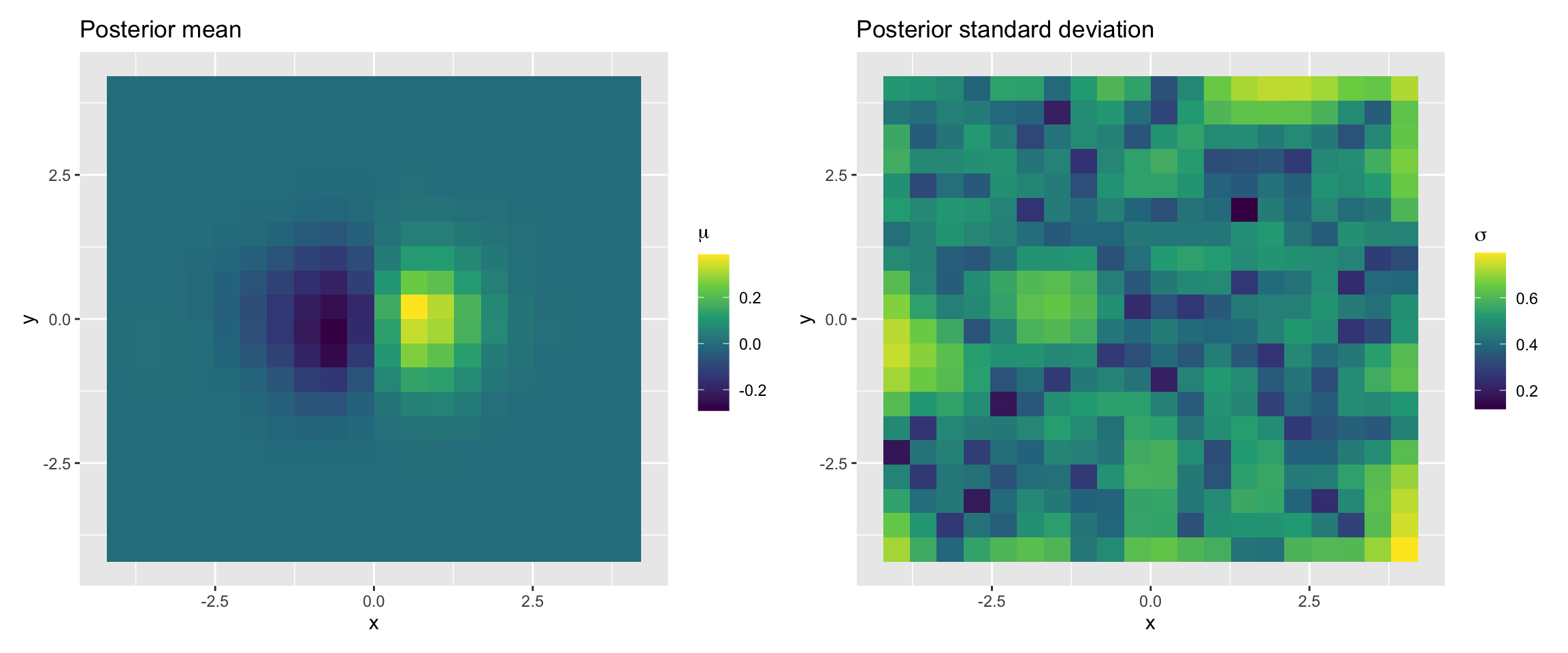

plot_ly(z = ~matrix(f(Z), ncol = 20)) |> add_surface()

plot_ly(z = matrix(results$z_m, ncol = 20)) |> add_surface()

References

Gramacy, Robert B. 2020. Surrogates: Gaussian Process Modeling, Design and  Optimization for the Applied Sciences. Boca Raton, Florida: Chapman Hall/CRC. https://bookdown.org/rbg/surrogates/.